Extragalactic Dusty Astrophysics at the University of Southampton

This is the official website of the CAT3D clumpy torus models as presented in Hönig & Kishimoto (2010). The model has recently been upgraded to include a more realistic dust sublimation model (differential dust sublimation depending on grain size and species) and account for the polar mid-IR emission seen in many nearby AGN (CAT3D-WIND; Hönig & Kishimoto 2017).
Contact: Any questions, suggestions, comments are welcome:

1. Summary and purpose

CAT3D and CAT3D-WIND provide model SEDs and images for the dusty environment around AGN. The dust is assumed to reside in clumps rather than being smoothly distributed. While CAT3D originally focused on the classical torus, CAT3D-WIND also includes dust in the polar outflow of the AGN. This adjustment was necessary since both infrared (IR) interferometry and single large telescopes detected strong mid-IR polar emission in many nearby AGN.
CAT3D combines Monte Carlo radiative transfer simulations and ray-tracing techniques through the clumpy environment in 3 dimensions, which makes the code relatively fast and suitable for parameter studies. The code will be able to capture statistical effects originating from the random distributuion of dust clouds according to a pre-specified set of model parameters. The model has been applied to a number of case and sample studies (see (4) CAT3D in action and (6) Work using CAT3D). SEDs are published below and images can be made accessible on request.

2. The method

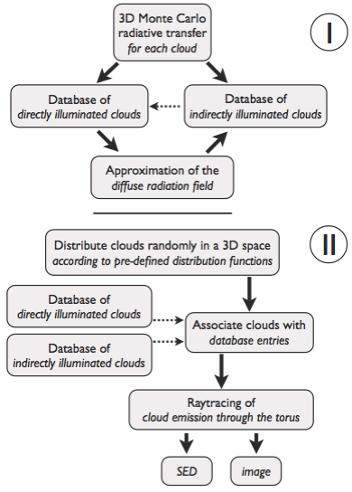
In a first step, the phaseangle-dependent emission for each cloud is simulated by Monte Carlo radiative transfer simulations. For that, the non-iterative local thermal equilibrium method by Bjorkman & Wood (2001) is applied, which is based on work by Lucy (1999). For each given dust composition, we determine the sublimation radius rsub=r(Tsub=1500K) from the source and simulate a database of clouds at different distances (normalized for rsub). Heating on each cloud is considered from the AGN (direct illumination) as well as the surrounding clouds (indirect illumination). To finally simulate the torus emission, dust clouds are distributed according to a set of parameters. Each distributed cloud is associated with a pre-simulated model cloud from the database, accounting for the individual cloud’s direct and indirect heating balance. The final torus image and SED is calculated via raytracing along the line-of-sight from each cloud to the observer. This method accounts for the actual 3-dimensional distribution of clouds in the distribution involving all statistical variations of randomly distributed clouds in a time-efficient way.

3. Model parameters

CAT3D and CAT3D-WIND have a range of model parameters, with the latter being an extension to the former. Indeed, CAT3D models can be reproduced by not distributing dust clouds in the polar region. The following provides an overview of the parameters. However, before using the model SEDs, please take the time and read Sect. 2.2 in Hönig & Kishimoto 2010 and Sect. 2 in Hönig & Kishimoto 2017 to fully understand their meaning.

torus/disk parameters (CAT3D and CAT3D-WIND)

• the index a of the radial dust cloud distribution power law
• the half-opening angle θ₀ (CAT3D) or, alternatively, the dimensionless scale heigh h = H/r (CAT3D-WIND)
• the number of clouds N₀ along an equatorial line-of-sight

wind parameters (only CAT3D-WIND)

• the index a_w of the dust cloud distribution power law along the wind
• the half-opening angle θ_w of the wind
• the angular width of the hollow wind cone σ_θ

global parameters (CAT3D and CAT3D-WIND)

• the ratio of dust clouds f_wd along the line-of-sight of the wind compared to the one in the disk plane (note: not to be confused for the mass ratio; see Hönig & Kishimoto 2017, Sect. 2 for a note on this; effectively f_wd=0 for CAT3D)
• the outer radius of the torus R_out (but see Sect. 4.1.4 in Hönig & Kishimoto 2010)
• the optical depth τ_cl of the individual clouds

4. Model downloads

The following model grids are available:

• CAT3D-WIND_SED_GRID.tar.gz: CAT3D-WIND model SED grid as presented in Hönig & Kishimoto 2017.
  
• CAT3D_SED_GRID.tar.gz: CAT3D model SED grid (without the wind) with the new implementation of the physical model for differential dust sublimation as presented in Hönig & Kishimoto 2017.
  


• CAT3D-WIND.IMAGES.GATOS.tar.gz: CAT3D-WIND model IMAGE grid with limited parameter space as used in GATOS paper II by Alonso-Herrero et al. 2021. Large file (8.4GB).
  


• CAT3D_torus_models_garcia17_isotropic.tar.gz: CAT3D torus model grid for isotropic AGN illumination as presented in Garcia et al. 2017. Each set of model parameters constains different SEDs for up to 10 random arrangement of dust clouds.
  
• CAT3D_torus_models_garcia17_anisotropic.tar.gz: CAT3D torus model grid for anisotropic AGN illumination as presented in Garcia et al. 2017. Each set of model parameters constains different SEDs for up to 10 random arrangement of dust clouds.
  

For legacy, the original model grid can also be downloaded:

• CAT3D.model_standard.tar.gz: This is the classical CAT3D torus grid of Hönig & Kishimoto 2010.

(Note section (5) How to cite CAT3D for terms of use of these models.)
Each model grid .tar.gz file consists of a number of ascii files. The ascii file names are referring to the model parameters used. Each file starts with a number of header lines (indicated by leading ‘#’) followed by 8 columns of data: col. 1 frequency (Hz); col. 2 wavelength (μm); col. 3-9 model νFν (W/m2) for inclination 0, 15, 30, 45, 60, 75, 90°.
The models are scaled in a way that they can be used for all kind of AGN. Nature does us a favor by setting an intrinsic scale for the torus: the dust sublimation radius which is depending on the luminosity. At this radius, the luminosity per unit area is always the same, no matter how powerful the AGN is. If we scale all of our sizes involved in the models for the dust sublimation radius, we are independent of the actual luminosity. Therefore the model fluxes are representing the emission that an observer at the distance of the sublimation radius would see. The conversion between model fluxes and observed fluxes is simply
where r_sub is the sublimation radius of the AGN you observe and D_L is the luminosity distance to the AGN. If you do not want to deal with the sublimation radius, it is also possible to use the AGN (optical/UV) luminosity instead because
r_sub;0 is depending on the dust which is used in the models and provided in the model description.

Examples:

1. We have a type 1 AGN at a distance of 45 Mpc with a sublimation radius (e.g. based on interferometry of IR reverberation mapping) is 0.06 pc. Our favorite model has a 12 μm model flux of 1.0 x 105 W/m². Thus, the prediction for the observed flux would be 1.78 x 10^-13 W/m² or 0.71 Jy.
2. Now, we have a type 2 AGN at a distance of 14.5 Mpc. It has a 12 μm model flux of 2.0 x 10⁴ W/m². In type 2s there’s no reverberation mapping which can measure rsub. However we can infer a UV luminosity by other means, let’s say log L = 44.5. Using the standard model (rsub;0 = 1.1 pc), we will obtain 3.64 x 10^-12 W/m² or 14.6 Jy.

5. How to cite CAT3D & CAT3D-WIND

Whenever you use the models provided here, please include the follwing references

for CAT3D: H\”onig, S. F., & Kishimoto, M. 2010, A&A, 523, 27

for CAT3D-WIND: H\”onig, S. F., & Kishimoto, M. 2017, ApJ, 838, L20

The original paper introducing the concept was:

H\”onig, S. F., Beckert, T., Ohnaka, K., & Weigelt, G. 2006, A&A, 452, 459.